I know it’s becoming a bit of a theme, but since I’ve briefly touched on statistics and how the query optimiser uses them for estimation, I thought I’d cover them in a bit more detail. How the query optimiser works is a very complicated topic that I may come back to at several points during this blog’s lifetime, but I think it’s worth having a good understanding of the basics when performing query optimisation.

Query Plan

SQL Server is a cost-based optimiser. What this means is that the query engine compares predicted costs of different ways to execute a query, then chooses the most efficient variation. The query engine estimates different query execution plans based on the statistics held on those particular objects in the database. Estimations are per execution, so if you take a look at the keylookup output in the execution plan below, you’ll see that the estimated number of rows is 1 whereas the actual is 38,868.

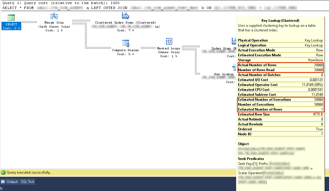
If we take a look at the properties of the keylookup in the picture above, we can see the number of executions was 38,868.

The point to remember is that estimation is not something that you should look at in isolation. The execution plan holds together as an entire entity, not as individual blocks. Another thing to note is that costs are not actual costs. By that, I mean that the cost has little or no relevance to actual execution costs. 1 cost does not mean anything, it is not a metric. Please do not rely on costs to determine the best plan.

Estimation Calculation

This is where the statistics come in. Statistics are automatically created and updated by the SQL Server optimiser, except in a few fringe cases. This can be done asynchronously (thankfully) and can be manually created or updated using T-SQL or management studio. Statistics are always against a column or columns, created automatically when an index is created or when you query columns from a table.

DBCC SHOW_STATISTICS({0},{1})

There are 4 options you can add to this, but if you do not pass any in then by default it will execute with stat_header, histogram, and density_vector which are the three that are important and supported by Microsoft.

WITH STAT_HEADER

This tells us the statistic name, the datetime it was last updated, the total number of rows, the total number of rows sampled (actually read to generate the statistic), the number of steps in the histogram (there can be a maximum of 200 steps), the density (rows / unique rows), average key length (this is the average byte length for all columns in the statistic) and finally the filtered rules.

WITH HISTOGRAM

Inside a histogram, each step contains data on a range of rows. The range is defined as being grater than the previous range_hi_key and less than or equal to the current range_hi_key.

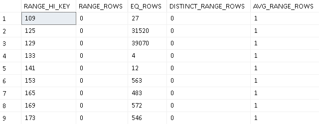
If you look at range_hi_key 129, what that data is representing is all rows that have a value greater than 125 but less than or equal to 129.

• EQ_ROWS - How many rows of data matched the range_hi_key from the sample
• RANGE_ROWS - How many rows of data matched the range from the sample
• DISTINCT_RANGE_ROWS - How many distinct rows matched the range from the sample
• AVG_RANGE_ROWS - The density of the data, e.g. RANGE_ROWS / DISTINCT_RANGE_ROWS

If we were to include a predicate filtering between 125 and 129 (i.e. WHERE X > 125 AND X <= 129), the execution plan looks like this: -

So when the query plan was generated, the query optimiser used the statistics held to estimate how many rows would fall in to the range that we looked at. If I don’t cheat and instead use a value or range in our predicate that does not appear in the statistics, for example a predicate filtering between 122 and 140, then SQL Server makes a guess based on the statistics it holds. In this case, because the average range rows is 1, it’s going to look at all of the rows in the statistics that fall between a range_hi_key of 122 and 140: -

• 125 - 31520
• 219 - 39070
• 133 - 4

It will then add up thoe figures, giving 70594: -

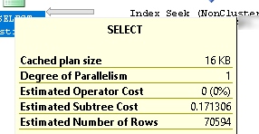
This makes it obvious that better query plans will come along when you have your statistically relevant keys in the “EQ_ROWS” and your non-statistically relevant (or less) in the ranges. This is worked out by the maxdiff algorithm, if you are not interested in statistical mathematics, then I wouldn’t bother researching it (and I certainly won’t be explaining it here!) as you can not change what the algorithm will return.

DROP TABLE IF EXISTS [testEnvironment];
  
SELECT TOP 500000
        IDENTITY( INT,1,1 ) AS [ID],
        ABS(CHECKSUM(NEWID())) AS [randomBigInt]
INTO    [testEnvironment]
FROM    [master].[sys].[syscolumns] [sc1]
CROSS JOIN [master].[sys].[syscolumns] [sc2]
CROSS JOIN [master].[sys].[syscolumns] [sc3];

CREATE CLUSTERED INDEX [cl_ID_testEnvironment] ON [testEnvironment] ([ID] ASC);
CREATE NONCLUSTERED INDEX [nc_randomBigInt_testEnvironment] ON [testEnvironment] ([randomBigInt] ASC);

INSERT  INTO [testEnvironment]
        ( [randomBigInt]
        )
SELECT TOP 500000
        ABS(CHECKSUM(NEWID())) AS [randomBigInt]
FROM    [master].[sys].[syscolumns] [sc1]
CROSS JOIN [master].[sys].[syscolumns] [sc2]
CROSS JOIN [master].[sys].[syscolumns] [sc3];

Above, I’ve created a million row test bed. After that, I executed: -

DBCC SHOW_STATISTICS([testEnvironment],[nc_randomBigInt_testEnvironment]) WITH HISTOGRAM;

As the sample data is pseudo-random, your results will not be identical to mine, but I have the following: -

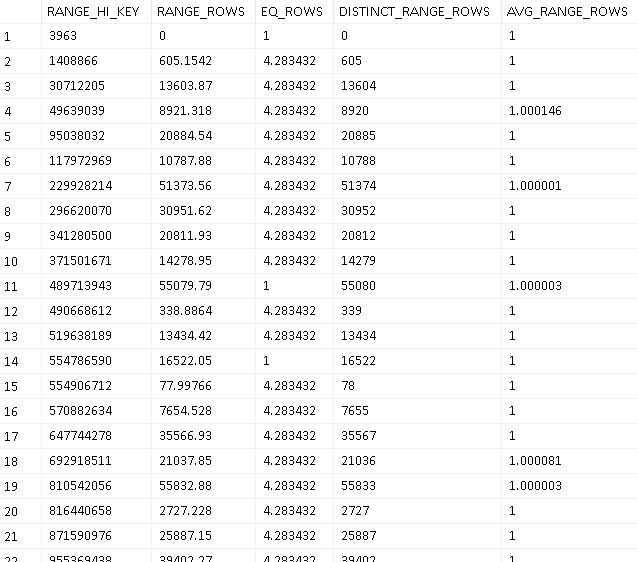
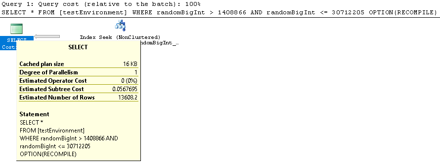
If we use the values from the range_hi_key in a predicate (i.e. WHERE randomBigInt > 1408866 AND randomBigInt <= 30712205), the estimate now uses trhe range_rows and the eq_rows (since both are greater than 0) to give us the estimate. In this case, 13603.87 + 4.283432, which gives us 13608.153432 so the execution plan will have estimated 13608.2: -

If we try a value that isn’t in the range_hi_key, e.g.

SELECT *
FROM [testEnvironment]
WHERE randomBigInt = 49639038
OPTION(RECOMPILE);

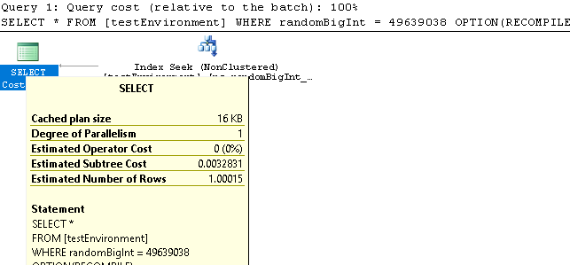
The query optimiser looks for the range_hi_key that this value falls in to and uses the avg_range_rows value for the estimate, in this case 1.000146 which will be rounded to 1.00015 in the graphical interface of the query plan: -

WITH DENSITY_VECTOR

This displays the density of columns (count of rows / count of distinct values).

For reference, we’re going to use the “nc_randomBigInt_testEnvironment” index defined above here.

So the index is on 1 columns, “randomBigInt”. Below is the result of the SHOW_STATISTICS on my system: -

All density	Average Length	Columns
1.000081E-06	4	randomBigInt
1E-06	8	randomBigInt, ID

So even though we have 1 column on the index, we get 2 columns in the density vector result-set. This is because the clustered index is part of the non-clustered index.

The first row above says that the density of the randomBigInt is 1.000081E-06, in other words COUNT OF ROWS / DISTINCT COUNT OF VALUES = 1.000081E-06. We could also use 1 / ROW DENSITY = DISTINCT COUNT OF VALUES, 1 / 1.000081E-06 = 999919.006560469 distinct values. If we run this: -

SELECT COUNT(*), COUNT(DISTINCT(randomBigInt)) FROM [testEnvironment];

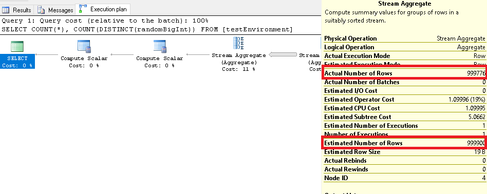
You can see in the execution plan where it estimated 999900 from the statistics, but the actual result was 999776.

Then finally, the second row tells us we are expecting 1000000 distinct values when including all of the columns from the index and the clustered index.

WITH STATS_STREAM

This displays the binary stats blob and is not supported by Microsoft. I include this only to mention that it exists, I’ve never used it so won’t be talking about it here.

Aged Statistics

To keep statistics relevant, they get “aged” which causes the statistics to be updated on next use (assuming you are automatically updating statistics), which in turn causes statements that are dependant on those statistics to be recompiled on next execution (rather than reusing the same execution plan). This happens at different intervals depending on the size of the table.

Table Size	Modifications Before Statistics “Aged”
0	Any modification / Insert
<= 500 Rows	500 modifications
>= 500 Rows	500 + 20% of table

Temporary tables in stored procedures behave differently. Normally, I’d discuss this in detail, but Paul White’s blog (specifically “Temporary Tables in Stored Procedures” and “Temporary Table Caching Explained”) goes in to a lot more detail than I ever could so I’m going to leave it and suggest you read his wonderful explanations.

There is a trace flag to change the threshold for large tables, since if you have a big table then 20% of the rows could be a high number of rows. So should we find that on a large table that we are having to manually update the statistics a lot, we can turn on trace flag 2371 which dynamically lowers the threshold for updating the statistics. Obviously this has the caveat of causing statements that depend on those statistics to be recompiled.

Filtered Statistics

When the density vector is not accurate enough, you can choose to manually create filtered statistics, e.g.

CREATE STATISTICS statsSmallNumbers ON dbo.testEnvironment([ID]) WHERE [randomBigInt] <= 10000;

DBCC SHOW_STATISTICS('testEnvironment', 'statsSmallNumbers') WITH STAT_HEADER;

Share on: